
HOME / POSTS / FPGA BEETHOVEN
FPGA Beethoven
November 2016 Love
Project Documents
I worked on this project with Mark Yang as our final project for 6.111 - Introductory Digital Systems Laboratory. Let's jump right in! Being able to hear what is on sheet music is very helpful to musicians beginning to learn a piece of music. Having auditory input can help people learn notes and rhythm more quickly and correct current mistakes. To make the transfer of sheet music to sound, we propose a digital music reading machine. This project will process a digital image of a score, and play the notes back to the user. There are two main parts to this project; note recognition (pitch and rhythm) and audio playback. This project starts with the reading of simple notes, rhythms and key signatures. If time permits, this project will evolve to read a score, notes that do not lie on the ledger lines, and music with accidentals. A user interface will allow the user to input the tempo and key signature of the piece before sight reading occurs.
High level overview
The digital sightreader takes an image of music stored in bRAM, processes it, and allows the user to listen to a digitized interpretation of the score. We begin with simple music, consisting only of quarter notes and half notes.

Figure 1. High level block diagram for the system.
Image formatting
Due to the limited time allotted to this project (approximately a month), the goal of this project was to provide a proof of concept that allows for expansion later on. Because of this, there is little flexibility for image uploads. This project assumes a .coe is available for upload to the labkit, where a black pixel is represented by a 0 and white pixel represented by a 1. Expansion later on could take an image provided by a camera hooked up to the labkit, or allow for image upload without having to reprogram the FPGA.
In order to generate a .coe file from a monochrome bitmap image, this matlab script was written. If the desired image of sheet music is formatted as a .jpg or .png, additional conversion must first be performed to produce a .bmp of the image. This can be done in matlab or using a third party image conversion program.
clc; close all;
[n,m] = size(image2);
fid = fopen('Keys.coe', 'w');
fprintf(fid, '%s\n', 'MEMORY_INITIALIZATION_RADIX=2;');
fprintf(fid, '%s\n', 'MEMORY_INITIALIZATION_VECTOR=');

for i = 1:n
    for j = 1:m
        fprintf(fid, '%s',char(image2(i,j) + 48));
        if (i == n && j == m)
            fprintf(fid,'%s',';');
        elseif (mod(j,m) == 0)
            fprintf(fid, '%s\n', ',');
        end
    end
end
fclose(fid);
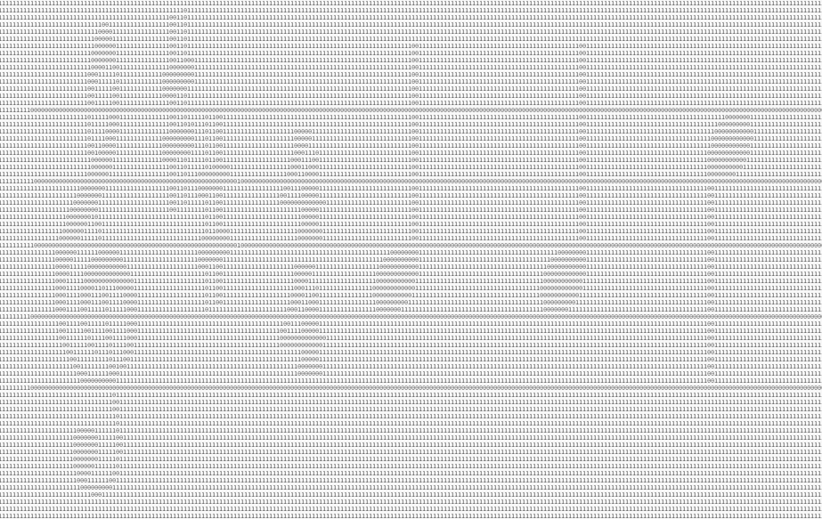
Figure 2. A .coe file that was produced using the matlab script above.
After the creation of a .coe file, the file can be uploaded to the bRAM on the lab kit. When initializing the image bRAM, the width of the bRAM should be equal to the width of the image in pixels and the depth should be equal to the height of the image. In our case, this was 901 pixels across, and 83 pixels tall.
Modules
Staff finder/line location finder
The purpose of this module is to determine where the lines of the staff lie on the image of the sheet music and to determine the spacing between each adjacent line. The staff finder module takes the staff detection user input data (vertical column of pixels) and determines the vertical spacing of the staff lines by calculating the number of white pixels between black pixels. Since notes also exists in between staffs, imaginary line locations are calculated to be between the staffs for later note detection.
The output of this module is an address pointer to the bRAM containing the original image. Each line of pixel is then sent back to this module for line detection. Wire arrays containing the locations of all lines and staffs become available to all modules after this initial analysis. The line locations provide the first step to convert the image into music.
Line eraser
The Line Eraser takes the locations of the staff from the globally available staff locations wire array, and removes these staff from the original image. This is done by taking in a line of pixels from the original image, then copying it to a new bRAM location dedicated for the line free image. The lines of pixels are copied exactly as they are in the original image, except for the lines that the staff resides on. A line of white pixels are saved in the corresponding address in the line free bRAM instead of the black staff lines. This step is taken to provide a clean base image of only the notes for the erosion and dilation modules. This can also serve as a debugging tool, as any error in line detection can be seen here. A comparison between the original image and the line erased image is shown below.


Figure 3. The original “Twinkle Twinkle Little Star” and the lined erased picture.
Note that since Verilog do not allow wire array inputs (for example, a bundle of 4 bit wide wires cannot be used as an input to a module), an extra step is taken to break up a long wire array within these modules to obtain the line location again. The line locations and staff locations are each packed into one long bundle of wires.
Dilation
The dilation and the erosion module are the backbone of our image processing approach. The dilation function thickens the lines and the notes. This function is applied to the original image repeatedly until the half notes become the same as the quarter notes - this is done to ensure that no half notes gets lost in the erosion process.
The implementation of this module utilizes a 3x3 convolution kernel. Essentially a pixel is picked as the center of this 3x3 matrix, and all pixels colors around the center pixel are compared against that of the center pixel. For dilation, if any pixel other than the center pixel in the 3x3 matrix is black, then the center pixel is written to be black.
This effectively expands the size of the notes. The below picture illustrates the dilation of the line erased picture.

Figure 4. Dilated notes. Note the half notes look identical to the quarter notes.
The dilation module sends out an address pointer to one of the two bRAMs holding the previously processed image (called frames). In return, it receives one line of pixels for processing. To looking through a 3x3 grid, 3 different rows of pixels need to be fetched and analyzed. After the image analysis, a new pixel is written to a buffer that holds a new line of pixel values. When this buffer is filled, the new line is written to the other processed image bRAM.

Figure 5: Dilation/Erosion module block diagram
Erosion
The erosion module is responsible for eliminating the stems of the notes. Erosion is one of two fundamental operations in morphological image processing (dilation being the other) and assigns the color white to any pixel not entirely surrounded by black pixels. Preliminary note detection will happen when the staff lines have been eroded (or removed) and before note heads have been entirely removed, and the size of the note heads is small enough such that it only overlaps one line.

Figure 6. Final processed image
The implementation of this module is similar to that of dilation. With the 3x3 matrix changed such that the center pixel is turned to white if any surrounding pixels within the 3x3 grid is white. A thing to note here is that erosion can be reversed by dilation, but when an isolated area is completely erased, dilation cannot restore the original image.
A tricky part about implementing the erosion and the dilation modules is dealing with off-by-one errors when the processed pixel line is saved to the bRAM. This caused a gradual shifting down of the processed image, which had to be corrected to ensure the correct function of the Note Mapper.
For the block diagram, please refer to the dilation section, as the inputs and the outputs are identical for these two modules, with the only difference being their internal processes.
Note detector/intersect detect
In music, horizontal location correlates to time and vertical position correlates to pitch. Note mapper takes the eroded image provided by the erosion module and determines the intersection between the note heads and the staff lines specified by the staff detection module. Knowing the vertical position of each note head provides information on what tone to play. Knowing which note is to the right of the note just processed provides information on when to play each note. It is the note mapper’s job to take each blob of black pixel from the erosion module and map it to a tone with a characteristic pitch and duration.
 Figure 7. Note Mapper detects the intersection of notes and lines
The implementation of the Note Mapper module on verilog uses a column-by-column approach. This means each column of pixels is checked against the line locations. If a row within the column contains a black pixel, and that row is the same as a row in the line locations list, then a note is detected. The line location is then sent to a bRAM holding all the line locations containing this intersection. Since the column-by-column approach checks columns from the left the right, the detected notes will already be in the correct temporal ordering. The audio modules can then access this notes storing bRAM for audio information.
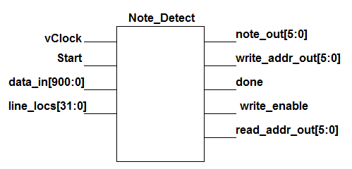
Figure 8. The Note Detection module block diagram. Note this block access two memory locations, one is the final processed image bRAM, the other is the bRAM that saves the note locations.
Muxes/address pointer select
Since each image processing module outputs their independent address pointers, the dual port RAM used to store various images will need to have their write enable ports, data in ports, and the data out ports connected to multiplexers switching between the different modules. This is done to ensure that the correct address and thus the data are fetched from the bRAMs and also to make the project more modular.
The output of these multiplexers are then toggled by the control FSM during each state transition. Both the pixel line data (901 bits wide) and the much shorter address data go through these muxes.
Image processing control FSM
Push buttons are used to go through states of image processing and analysis for demonstration purposes, since the FPGA is very fast at performing the algorithms in this project, it is impossible to see the steps of the process if the processes are to be triggered by the program itself.
A specific sequence of dilation and erosion is used to ensure that the end image contains the note heads that are the right size (only intersect with one line) for note detection. This specific sequence is:
Dilate -> Dilate (at this point, quarter notes and half notes look identical) -> erode x 5
For future improvements, it is very possible to make the program automatically detect the dilation and erosion sequence needed to produce the optimal final result for note detection.
Sequence for walking through FSM - Note initial position of switches must be flipped towards the user:
>> Button 0
>> Switch 7
>> Button 3
>> Switch 6
>> Button 1
>> Switch 5
>> Keep pressing Button 1 until erosion completes.
At any point in this process, if the up button is pressed, rhythm data will be written to the rhythm bRAM and the piece will then be played in correct rhythm.
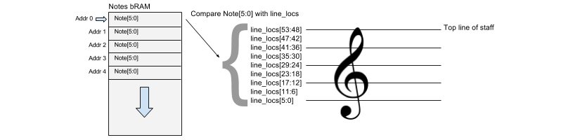
If the Note[5:0] (see Figure 11) data coming from the notes bRAM does not match any of the locations stored in line_locs[53:0], the default tone of D#4/Eb4 is played. When going through the control FSM stated above, typical playback is as follows:
Note 0 (F#5/Gb5) - or Note 1 (F5), depending on key signature until line_locs is filled (line_locs is initialized with 0)
Note 15 (D#4/Eb4) - Notes bRAM has not been filled with data yet thus Note[5:0] does not match any data in line_locs[53:0]. When there is no data match, default is note is 15.
After all erosion happens, Note[5:0] maps to data in line_loc[53:0] and music is played (in or out of rhythm depending if the up button has been pressed.)
All these tones are played as half notes until the up button is pressed and the rhythm bram is filled with useful data. Rhythm bRAM is initialized with 0’s hence why default rhythm is a half note.
Display image
This is the main image module that is responsible for displaying most of the images on the screen.
A problem here is that the display module uses a different number of sequenced non-blocking statements than a separate module that displays the keys. This caused display glitches. An effort to implement a two stage pipeline solved this issue by allowing enough time for pixel logic to be computed.
Display keys
Display Keys module is a simple module that displays a .coe file stored in bram. This image provides a graphical user interface that allows the user to specify the key in which the piece is played.
Blob - key selector blob
Blob is a rectangle that overlaps the Key image that allows the user select the key signature of the piece. The pixels from this module are alpha blended with the pixels from the Display Keys module to provide a blend of approximately 50/50. The x and y locations of this blob are controlled by the up, down, left and right buttons on the labkit.
Lab5audio
The lab5audio module is a module that was taken from lab 5 and inserted to handle the interface between our code and the AC97 chip on the labkit.
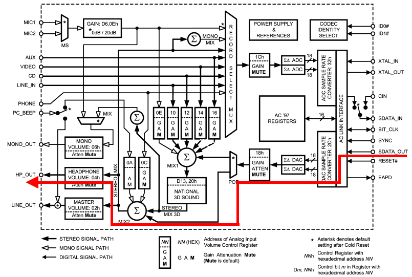
Figure 9. Data path of outgoing audio to headphones.
FROM LAB 5:
the FPGA transmits a 256-bit frame of serial data to the AC97 chip via the SDATA-OUT pin. Each frame contains two 18-bit fields with PCM data for the left and right audio channels. The PCM data is converted to two 48kHz analog waveforms by the sigma-delta digital-to- analog converters (ΣΔDACs). The analog waveforms are amplified and sent to the stereo headphones.
48,000 times per second the AC97 codec provides two stereo PCM samples from the microphone and accepts two stereo PCM samples for the headphones. It's the FPGA's job to keep up with the codec's data rates since the codec does not have on-chip buffering for either the incoming or outgoing data streams.
Notes
The notes module supplies a 20-bit PCM stream to the AC97 Audio Codec chip (LM4550) on the labkit. Currently there are 16 notes that range from D#4/Eb4 (lowest note on the staff) to F#5/Gb5 (highest note on the staff). Data for each note is stored in a case statement that maps a note input to the appropriate PCM data samples. The AC97 samples the data from this module at 48KHz. In order to achieve an output tone of A4 (440Hz), there must be 109 PCM data samples (48,000Hz / 440Hz) that map out one period of a sine wave. Number of PCM data samples for other notes are displayed in the table below.
|
NOTE |
FREQUECY (Hz) |
# OF SAMPLES |
ROUNDED |
INDEX RANGE |
|
F#5/Gb5 |
739.99 |
64.86574143 |
65 |
0 - 64 |
|
F5 |
698.46 |
68.72261833 |
69 |
0 - 68 |
|
E5 |
659.25 |
72.81001138 |
73 |
0 -72 |
|
D#5/Eb5 |
622.25 |
77.13941342 |
77 |
0 - 76 |
|
D5 |
587.33 |
81.72577597 |
82 |
0 - 81 |
|
C#5/Db5 |
554.37 |
86.5847719 |
87 |
0 - 86 |
|
C5 |
523.25 |
91.7343526 |
92 |
0 -91 |
|
B4 |
493.88 |
97.18960071 |
97 |
0 - 96 |
|
A#4/Bb4 |
466.16 |
102.9689377 |
103 |
0 - 102 |
|
A4 |
440 |
109.0909091 |
109 |
0 - 108 |
|
G#4/Ab4 |
415.3 |
115.5790994 |
116 |
0 - 115 |
|
G4 |
392 |
122.4489796 |
122 |
0 - 121 |
|
F#4/Gb4 |
369.99 |
129.733236 |
130 |
0 - 129 |
|
F4 |
349.23 |
137.4452367 |
137 |
0 - 136 |
|
E4 |
329.63 |
145.6178139 |
146 |
0 - 145 |
|
D#4/Eb4 |
311.13 |
154.2763475 |
154 |
0 - 153 |
Figure 10. Number of pcm data sample for each tone for ac97.
All tones played by the labkit in this project are pure sine waves with no harmonics or overtones. Future improvement could include looking at the frequency response of various instruments and trying to mimic the characteristic sound of a few by having the labkit play higher harmonics.
Note mapper
Note mapper is the module that maps the location of each notehead to a number that corresponds to an output tone. Note mapper takes in an array (line_locs) from staff detection module that contains the location of each staff line and space. Note mapper then addresses through the bRAM that stores the location of each notehead and compares that location to the staff locations specified in line_locs.
Figure 11. Note mapping.
The note mapper module primarily comprises of nested case statements. One case statement handles the key and the other handles mapping a pixel location of note to a numerical, 4 bit number. See below for how notes are coded.
|
NOTE |
CODE/NUMERICAL VALUE |
|
|
F#5/Gb5 |
0 |
4'b0000 |
|
F5 |
1 |
4'b0001 |
|
E5 |
2 |
4'b0010 |
|
D#5/Eb5 |
3 |
4'b0011 |
|
D5 |
4 |
4'b0100 |
|
C#5/Db5 |
5 |
4'b0101 |
|
C5 |
6 |
4'b0110 |
|
B4 |
7 |
4'b0111 |
|
A#4/Bb4 |
8 |
4'b1000 |
|
A4 |
9 |
4'b1001 |
|
G#4/Ab4 |
10 |
4'b1010 |
|
G4 |
11 |
4'b1011 |
|
F#4/Gb4 |
12 |
4'b1100 |
|
F4 |
13 |
4'b1101 |
|
E4 |
14 |
4'b1110 |
|
D#4/Eb4 |
15 (default) |
4'b1111 |
Figure 12. Note codes.
Play music
Play Music takes in all the necessary lines that are needed to play the music. Inputs and outputs include beat, note (a 4 bit value that comes out of the note mapper module), and address pointers that control the data on rhythm wires that tell the play music module the duration of each note that is to be played. This module is also where the length of the piece is set. Once the pitch and rhythm of each note has been determined, the play music module continuously loops through the music over and over again. To distinguish the beginning of one note from the end of the previous note, the play music decrements the volume of playback so that a note has a natural decay to it, as if striking a key on a piano with an initial impulse then decay in volume. The rate of volume decrease for each note is fixed no matter the rhythmic value of the note. This most closely mimics the decay in volume when a piano key is struck.
Key selector
The Key Selector module reads the location of the key cursor (blob) and maps that location to a specific key. Below is a table that contains the X and Y location of the selector blob for each key signature . For example, if the key selector blob has an X pixel location of 51 and a Y pixel location of 47, this will set the key to D major. The key can be set by the user that differs than the actually key of the sheet music upload to allow for interesting music playback.
|
D |
E |
F |
G |
A |
B |
|
X: 51 |
X: 134 |
X: 217 |
X: 300 |
X: 383 |
X: 466 |
|
Y: 47 |
Y: 47 |
Y: 47 |
Y: 47 |
Y: 47 |
Y: 47 |
|
Db |
Eb |
F# |
Gb |
Ab |
Bb |
|
X: 51 |
X: 134 |
X: 217 |
X: 300 |
X: 383 |
X: 466 |
|
Y: 158 |
Y: 158 |
Y: 158 |
Y: 158 |
Y: 158 |
Y: 158 |
Figure 13. Pixel map of key selector.
User metronome
Since some music has a faster tempo (i.e. speed) than others, a metronome module was built to adjust the bpm (beats per minute) of the tempo module. The user can adjust the bmp of playback by pressing button 2 on the labkit. If switch 0 is high and button 2 is pressed, bpm is increased by 5. If switch 0 is low and button 2 is pressed, bpm is decreased by 5. The slowest bmp the user can set is 40 bpm and the highest is 180 bpm. These maximum and minimum bpm values are arbitrary and can be adjusted by more code. Most music falls within this tempo range.
Tempo
Tempo provides a pulse that corresponds the the bmp set by user metronome. For example, if the user has set the bmp of playback to 100 bpm (default), tempo will provide a pulse with a frequency of 100 times per minute on the wire beat[0:0]. This pulse is high for one period of a 65mHz clock line and low for the rest. This beat corresponds to a quarter note, and thus must be further subdivided in order to play faster rhythms, such as 18th notes and 16th notes (not done in this iteration of the project).
Pixel integration
This module handles almost all of the rhythm detection for this project and in essence is one large state machine. The states are SUM_COLUMNS, PAUSE, INTEGRATE, WAIT, MAP, RECOVER, and DRAW.
SUM_COLUMNS
SUM_COLUMNS does a sweep across the columns of pixels of the image of sheet music stored in bRAM and while doing so, adds the number of black pixels it “sees” in each column. The result is written to separate bram that stores this data to be used by the INTEGRATE state of this FSM.
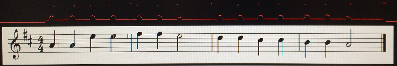
Figure 14. Data in bRAM (red) from counting number of black pixels in each column.
PAUSE
Sets addresses and write enable lines for bRAM to get ready for the INTEGRATE state.
INTEGRATE
The integrate state takes data from summing the number of black pixels in each column and adds up each group of pixels that rise above the 5 pixel line (5 pixels as there are 5 staff lines, each one pixel tall). This is the process: when a column count is registered as greater than 5, the INTEGRATE state accumulates all the following data until pixel count falls back to 5. This data is saved in bRAM and the data write address is increment for the next note. The result of adding up all the pixels in each note is shown below in Figure 15.
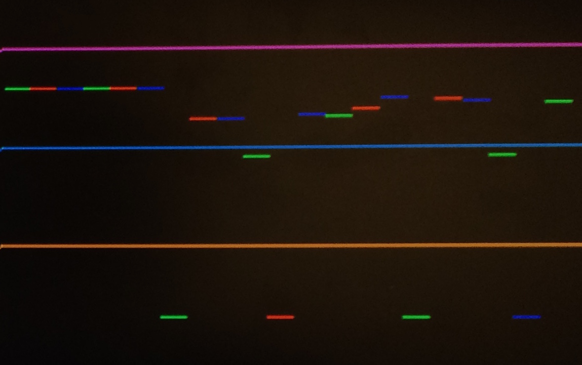
Figure 15. Data in bRAM from adding number of black pixels in each note.
WAIT
WAIT plays a similar role as the PAUSE state: WAIT initializes write enable and address lines such that they are ready for MAPPING
MAP
MAP maps each value stored in the integration bRAM to a rhythmic note depending on where it falls within specified thresholds (thresholds are visible in Figure 16 as solid pink, blue and orange lines). These thresholds are set by the user/programmer.
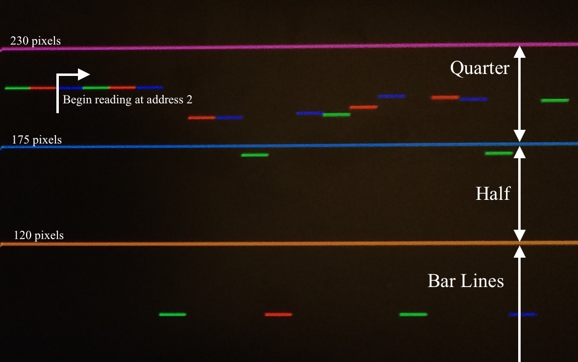
Figure 16. Annotated data in bRAM from adding number of black pixels in each note.
There are discrepancies between the values of some of the quarter notes shown in the figure above. This is due to the fact that some noteheads land in a space on the staff, and others on a line. Notes that fall in a space have a higher pixel count than notes that fall on a line.
RECOVER
RECOVER “recovers” the initial state of all the necessary address lines and increments other addresses depending on if data writes have happened. RECOVER also checks if all notes have been accounted for (number of notes is specified by user/programmer) and if so, transitions to the DRAW state.
DRAW
The DRAW state “draws” out data stored in bRAM so it is viewable by the user/programmer and displays it of the VGA display. This state is entirely for debugging and presentation purposes. Figure 15 and 16 are the visuals this state produces.
Discussion and conclusion
We were successful in providing a proof of concept for this idea that can certainly be expanded upon in the future. There are some downsides to the current technique of detecting rhythm and one must be wary of the fact that notes with the same rhythm can come in many different forms that may vary in pixel count.
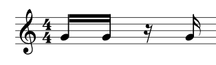
Figure 17. Different shapes that all need to be mapped to a value of a 16th note
In addition, by just relying on the number of black pixels in each note, information is lost, most importantly, the shape of the note. It is also difficult to detect the end of the piece as one can see from Figure 16 that the thick vertical line at the end of the piece has a similar pixel count as a quarter note, and thus is indistinguishable from a quarter note with this current recognition technique. Therefore it is necessary for the user to manually input the number of notes of the score so the FPGA knows when to stop detecting rhythm. One benefit the counting pixel method provides however is very clear and consistent bar line readings. Looking at Figure 16, one can clearly see that bar lines have very little pixel variation and fall far from the pixel count of any of the notes tested so far. This makes them very easy to detect by the FPGA. One can leverage this by using bar lines as a way to “parity check” the pixel values that get mapped to rhythmic values. For example, if the time signature is 4/4, there will always be 4 beats per measure, where the quarter note gets the beat. Therefore, if more than 4 beats are detected in a measure, a flag should be raised and the note closest to a threshold should be changed in order to fix the beats per measure to 4. While this parity check was not implemented in this version of the project, it is something that could be very useful for future revisions or other projects of this sort. This project also assumed no chords were present in the score, where a chord is a stack of notes meant to be played simultaneously. In most cases, music is polyphonic, where there is more than just one line playing at a single time. The erosion and dilation should be able to handle this well, however, this may throw of rhythm detection, especially when notes of different rhythmic values are stacked on top of each other. The easiest way to handle this would be to require the upload of a single voice/line at a time and process until all voices have been read. Again, something to be considered for the future.